Python Fundamentals

Overview

Teaching: 20 min
Exercises: 0 min

Questions

• What basic data types can I work with in Python?

• How can I create a new variable in Python?

• Can I change the value associated with a variable after I create it?

Objectives

• Assign values to variables.

Variables

Any Python interpreter can be used as a calculator:

3 + 5 * 4

23

This is great but not very interesting. To do anything useful with data, we need to assign its value to a variable. In Python, we can assign a value to a variable, using the equals sign =. For example, to assign value 60 to a variable weight_kg, we would execute:

weight_kg = 60

From now on, whenever we use weight_kg, Python will substitute the value we assigned to it. In layman’s terms, a variable is a name for a value.

In Python, variable names:

• can include letters, digits, and underscores
• cannot start with a digit
• are case sensitive.

This means that, for example:

• weight0 is a valid variable name, whereas 0weight is not
• weight and Weight are different variables

Types of data

Python knows various types of data. Three common ones are:

• integer numbers
• floating point numbers, and
• strings.

In the example above, variable weight_kg has an integer value of 60. To create a variable with a floating point value, we can execute:

weight_kg = 60.0

And to create a string, we add single or double quotes around some text, for example:

weight_kg_text = 'weight in kilograms:'

Using Variables in Python

To display the value of a variable to the screen in Python, we can use the print function:

print(weight_kg)

60.0

We can display multiple things at once using only one print command:

print(weight_kg_text, weight_kg)

weight in kilograms: 60.0

Moreover, we can do arithmetic with variables right inside the print function:

print('weight in pounds:', 2.2 * weight_kg)

weight in pounds: 132.0

The above command, however, did not change the value of weight_kg:

print(weight_kg)

60.0

To change the value of the weight_kg variable, we have to assign weight_kg a new value using the equals = sign:

weight_kg = 65.0
print('weight in kilograms is now:', weight_kg)

weight in kilograms is now: 65.0

Variables as Sticky Notes

A variable is analogous to a sticky note with a name written on it: assigning a value to a variable is like putting that sticky note on a particular value.

This means that assigning a value to one variable does not change values of other variables. For example, let’s store the subject’s weight in pounds in its own variable:

# There are 2.2 pounds per kilogram
weight_lb = 2.2 * weight_kg
print(weight_kg_text, weight_kg, 'and in pounds:', weight_lb)

weight in kilograms: 65.0 and in pounds: 143.0

Let’s now change weight_kg:

weight_kg = 100.0
print('weight in kilograms is now:', weight_kg, 'and weight in pounds is still:', weight_lb)

weight in kilograms is now: 100.0 and weight in pounds is still: 143.0

Since weight_lb doesn’t “remember” where its value comes from, it is not updated when we change weight_kg.

Key Points

• Basic data types in Python include integers, strings, and floating-point numbers.

• Use variable = value to assign a value to a variable in order to record it in memory.

• Variables are created on demand whenever a value is assigned to them.

• Use print(something) to display the value of something.

Analyzing Patient Data

Overview

Teaching: 40 min
Exercises: 20 min

Questions

• How can I process tabular data files in Python?

Objectives

• Explain what a library is and what libraries are used for.

• Import a Python library and use the functions it contains.

• Read tabular data from a file into a program.

• Select individual values and subsections from data.

• Perform operations on arrays of data.

Words are useful, but what’s more useful are the sentences and stories we build with them. Similarly, while a lot of powerful, general tools are built into Python, specialized tools built up from these basic units live in libraries that can be called upon when needed.

Loading data into Python

To begin processing inflammation data, we need to load it into Python. We can do that using a library called NumPy, which stands for Numerical Python. In general, you should use this library when you want to do fancy things with lots of numbers, especially if you have matrices or arrays. To tell Python that we’d like to start using NumPy, we need to import it:

import numpy

Importing a library is like getting a piece of lab equipment out of a storage locker and setting it up on the bench. Libraries provide additional functionality to the basic Python package, much like a new piece of equipment adds functionality to a lab space. Just like in the lab, importing too many libraries can sometimes complicate and slow down your programs - so we only import what we need for each program.

Once we’ve imported the library, we can ask the library to read our data file for us:

numpy.loadtxt(fname='inflammation-01.csv', delimiter=',')

array([[ 0.,  0.,  1., ...,  3.,  0.,  0.],
       [ 0.,  1.,  2., ...,  1.,  0.,  1.],
       [ 0.,  1.,  1., ...,  2.,  1.,  1.],
       ...,
       [ 0.,  1.,  1., ...,  1.,  1.,  1.],
       [ 0.,  0.,  0., ...,  0.,  2.,  0.],
       [ 0.,  0.,  1., ...,  1.,  1.,  0.]])

The expression numpy.loadtxt(...) is a function call that asks Python to run the function loadtxt which belongs to the numpy library. This dotted notation is used everywhere in Python: the thing that appears before the dot contains the thing that appears after.

As an example, John Smith is the John that belongs to the Smith family. We could use the dot notation to write his name smith.john, just as loadtxt is a function that belongs to the numpy library.

numpy.loadtxt has two parameters: the name of the file we want to read and the delimiter that separates values on a line. These both need to be character strings (or strings for short), so we put them in quotes.

Since we haven’t told it to do anything else with the function’s output, the notebook displays it. In this case, that output is the data we just loaded. By default, only a few rows and columns are shown (with ... to omit elements when displaying big arrays). Note that, to save space when displaying NumPy arrays, Python does not show us trailing zeros, so 1.0 becomes 1..

Our call to numpy.loadtxt read our file but didn’t save the data in memory. To do that, we need to assign the array to a variable. In a similar manner to how we assign a single value to a variable, we can also assign an array of values to a variable using the same syntax. Let’s re-run numpy.loadtxt and save the returned data:

data = numpy.loadtxt(fname='inflammation-01.csv', delimiter=',')

This statement doesn’t produce any output because we’ve assigned the output to the variable data. If we want to check that the data have been loaded, we can print the variable’s value:

print(data)

[[ 0.  0.  1. ...,  3.  0.  0.]
 [ 0.  1.  2. ...,  1.  0.  1.]
 [ 0.  1.  1. ...,  2.  1.  1.]
 ...,
 [ 0.  1.  1. ...,  1.  1.  1.]
 [ 0.  0.  0. ...,  0.  2.  0.]
 [ 0.  0.  1. ...,  1.  1.  0.]]

Now that the data are in memory, we can manipulate them. First, let’s ask what type of thing data refers to:

print(type(data))

<class 'numpy.ndarray'>

The output tells us that data currently refers to an N-dimensional array, the functionality for which is provided by the NumPy library. These data correspond to arthritis patients’ inflammation. The rows are the individual patients, and the columns are their daily inflammation measurements.

Data Type

A Numpy array contains one or more elements of the same type. The type function will only tell you that a variable is a NumPy array but won’t tell you the type of thing inside the array. We can find out the type of the data contained in the NumPy array.

print(data.dtype)

float64

This tells us that the NumPy array’s elements are floating-point numbers.

With the following command, we can see the array’s shape:

print(data.shape)

(60, 40)

The output tells us that the data array variable contains 60 rows and 40 columns. When we created the variable data to store our arthritis data, we did not only create the array; we also created information about the array, called members or attributes. This extra information describes data in the same way an adjective describes a noun. data.shape is an attribute of data which describes the dimensions of data. We use the same dotted notation for the attributes of variables that we use for the functions in libraries because they have the same part-and-whole relationship.

If we want to get a single number from the array, we must provide an index in square brackets after the variable name, just as we do in math when referring to an element of a matrix. Our inflammation data has two dimensions, so we will need to use two indices to refer to one specific value:

print('first value in data:', data[0, 0])

first value in data: 0.0

print('middle value in data:', data[30, 20])

middle value in data: 13.0

The expression data[30, 20] accesses the element at row 30, column 20. While this expression may not surprise you, data[0, 0] might. Programming languages like Fortran, MATLAB and R start counting at 1 because that’s what human beings have done for thousands of years. Languages in the C family (including C++, Java, Perl, and Python) count from 0 because it represents an offset from the first value in the array (the second value is offset by one index from the first value). This is closer to the way that computers represent arrays (if you are interested in the historical reasons behind counting indices from zero, you can read Mike Hoye’s blog post). As a result, if we have an M×N array in Python, its indices go from 0 to M-1 on the first axis and 0 to N-1 on the second. It takes a bit of getting used to, but one way to remember the rule is that the index is how many steps we have to take from the start to get the item we want.

In the Corner

What may also surprise you is that when Python displays an array, it shows the element with index [0, 0] in the upper left corner rather than the lower left. This is consistent with the way mathematicians draw matrices but different from the Cartesian coordinates. The indices are (row, column) instead of (column, row) for the same reason, which can be confusing when plotting data.

Slicing data

An index like [30, 20] selects a single element of an array, but we can select whole sections as well. For example, we can select the first ten days (columns) of values for the first four patients (rows) like this:

print(data[0:4, 0:10])

[[ 0.  0.  1.  3.  1.  2.  4.  7.  8.  3.]
 [ 0.  1.  2.  1.  2.  1.  3.  2.  2.  6.]
 [ 0.  1.  1.  3.  3.  2.  6.  2.  5.  9.]
 [ 0.  0.  2.  0.  4.  2.  2.  1.  6.  7.]]

The slice 0:4 means, “Start at index 0 and go up to, but not including, index 4”. Again, the up-to-but-not-including takes a bit of getting used to, but the rule is that the difference between the upper and lower bounds is the number of values in the slice.

We don’t have to start slices at 0:

print(data[5:10, 0:10])

[[ 0.  0.  1.  2.  2.  4.  2.  1.  6.  4.]
 [ 0.  0.  2.  2.  4.  2.  2.  5.  5.  8.]
 [ 0.  0.  1.  2.  3.  1.  2.  3.  5.  3.]
 [ 0.  0.  0.  3.  1.  5.  6.  5.  5.  8.]
 [ 0.  1.  1.  2.  1.  3.  5.  3.  5.  8.]]

We also don’t have to include the upper and lower bound on the slice. If we don’t include the lower bound, Python uses 0 by default; if we don’t include the upper, the slice runs to the end of the axis, and if we don’t include either (i.e., if we use ‘:’ on its own), the slice includes everything:

small = data[:3, 36:]
print('small is:')
print(small)

The above example selects rows 0 through 2 and columns 36 through to the end of the array.

small is:
[[ 2.  3.  0.  0.]
 [ 1.  1.  0.  1.]
 [ 2.  2.  1.  1.]]

Analyzing data

NumPy has several useful functions that take an array as input to perform operations on its values. If we want to find the average inflammation for all patients on all days, for example, we can ask NumPy to compute data’s mean value:

print(numpy.mean(data))

6.14875

mean is a function that takes an array as an argument.

Not All Functions Have Input

Generally, a function uses inputs to produce outputs. However, some functions produce outputs without needing any input. For example, checking the current time doesn’t require any input.

import time
print(time.ctime())

Sat Mar 26 13:07:33 2016

For functions that don’t take in any arguments, we still need parentheses (()) to tell Python to go and do something for us.

Let’s use three other NumPy functions to get some descriptive values about the dataset. We’ll also use multiple assignment, a convenient Python feature that will enable us to do this all in one line.

maxval, minval, stdval = numpy.max(data), numpy.min(data), numpy.std(data)

print('maximum inflammation:', maxval)
print('minimum inflammation:', minval)
print('standard deviation:', stdval)

Here we’ve assigned the return value from numpy.max(data) to the variable maxval, the value from numpy.min(data) to minval, and so on.

maximum inflammation: 20.0
minimum inflammation: 0.0
standard deviation: 4.61383319712

Mystery Functions in IPython

How did we know what functions NumPy has and how to use them? If you are working in IPython or in a Jupyter Notebook, there is an easy way to find out. If you type the name of something followed by a dot, then you can use tab completion (e.g. type numpy. and then press Tab) to see a list of all functions and attributes that you can use. After selecting one, you can also add a question mark (e.g. numpy.cumprod?), and IPython will return an explanation of the method! This is the same as doing help(numpy.cumprod). Similarly, if you are using the “plain vanilla” Python interpreter, you can type numpy. and press the Tab key twice for a listing of what is available. You can then use the help() function to see an explanation of the function you’re interested in, for example: help(numpy.cumprod).

When analyzing data, though, we often want to look at variations in statistical values, such as the maximum inflammation per patient or the average inflammation per day. One way to do this is to create a new temporary array of the data we want, then ask it to do the calculation:

patient_0 = data[0, :] # 0 on the first axis (rows), everything on the second (columns)
print('maximum inflammation for patient 0:', numpy.max(patient_0))

maximum inflammation for patient 0: 18.0

Everything in a line of code following the ‘#’ symbol is a comment that is ignored by Python. Comments allow programmers to leave explanatory notes for other programmers or their future selves.

We don’t actually need to store the row in a variable of its own. Instead, we can combine the selection and the function call:

print('maximum inflammation for patient 2:', numpy.max(data[2, :]))

maximum inflammation for patient 2: 19.0

What if we need the maximum inflammation for each patient over all days (as in the next diagram on the left) or the average for each day (as in the diagram on the right)? As the diagram below shows, we want to perform the operation across an axis:

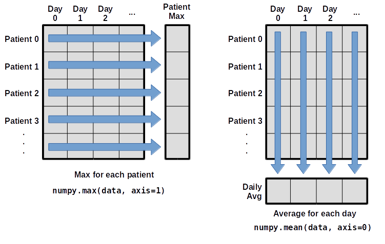
To support this functionality, most array functions allow us to specify the axis we want to work on. If we ask for the average across axis 0 (rows in our 2D example), we get:

print(numpy.mean(data, axis=0))

[  0.           0.45         1.11666667   1.75         2.43333333   3.15
   3.8          3.88333333   5.23333333   5.51666667   5.95         5.9
   8.35         7.73333333   8.36666667   9.5          9.58333333
  10.63333333  11.56666667  12.35        13.25        11.96666667
  11.03333333  10.16666667  10.           8.66666667   9.15         7.25
   7.33333333   6.58333333   6.06666667   5.95         5.11666667   3.6
   3.3          3.56666667   2.48333333   1.5          1.13333333
   0.56666667]

As a quick check, we can ask this array what its shape is:

print(numpy.mean(data, axis=0).shape)

(40,)

The expression (40,) tells us we have an N×1 vector, so this is the average inflammation per day for all patients. If we average across axis 1 (columns in our 2D example), we get:

print(numpy.mean(data, axis=1))

[ 5.45   5.425  6.1    5.9    5.55   6.225  5.975  6.65   6.625  6.525
  6.775  5.8    6.225  5.75   5.225  6.3    6.55   5.7    5.85   6.55
  5.775  5.825  6.175  6.1    5.8    6.425  6.05   6.025  6.175  6.55
  6.175  6.35   6.725  6.125  7.075  5.725  5.925  6.15   6.075  5.75
  5.975  5.725  6.3    5.9    6.75   5.925  7.225  6.15   5.95   6.275  5.7
  6.1    6.825  5.975  6.725  5.7    6.25   6.4    7.05   5.9  ]

which is the average inflammation per patient across all days.

Key Points

• Import a library into a program using import libraryname.

• Use the numpy library to work with arrays in Python.

• The expression array.shape gives the shape of an array.

• Use array[x, y] to select a single element from a 2D array.

• Array indices start at 0, not 1.

• Use low:high to specify a slice that includes the indices from low to high-1.

• Use # some kind of explanation to add comments to programs.

• Use numpy.mean(array), numpy.max(array), and numpy.min(array) to calculate simple statistics.

• Use numpy.mean(array, axis=0) or numpy.mean(array, axis=1) to calculate statistics across the specified axis.

Visualizing Tabular Data

Overview

Teaching: 30 min
Exercises: 20 min

Questions

• How can I visualize tabular data in Python?

• How can I group several plots together?

Objectives

• Plot simple graphs from data.

• Group several graphs in a single figure.

Visualizing data

The mathematician Richard Hamming once said, “The purpose of computing is insight, not numbers,” and the best way to develop insight is often to visualize data. Visualization deserves an entire lecture of its own, but we can explore a few features of Python’s matplotlib library here. While there is no official plotting library, matplotlib is the de facto standard. First, we will import the pyplot module from matplotlib and use two of its functions to create and display a heat map of our data:

import matplotlib.pyplot
image = matplotlib.pyplot.imshow(data)
matplotlib.pyplot.show()

Blue pixels in this heat map represent low values, while yellow pixels represent high values. As we can see, inflammation rises and falls over a 40-day period. Let’s take a look at the average inflammation over time:

ave_inflammation = numpy.mean(data, axis=0)
ave_plot = matplotlib.pyplot.plot(ave_inflammation)
matplotlib.pyplot.show()

Here, we have put the average inflammation per day across all patients in the variable ave_inflammation, then asked matplotlib.pyplot to create and display a line graph of those values. The result is a roughly linear rise and fall, which is suspicious: we might instead expect a sharper rise and slower fall. Let’s have a look at two other statistics:

max_plot = matplotlib.pyplot.plot(numpy.max(data, axis=0))
matplotlib.pyplot.show()

min_plot = matplotlib.pyplot.plot(numpy.min(data, axis=0))
matplotlib.pyplot.show()

The maximum value rises and falls smoothly, while the minimum seems to be a step function. Neither trend seems particularly likely, so either there’s a mistake in our calculations or something is wrong with our data. This insight would have been difficult to reach by examining the numbers themselves without visualization tools.

Grouping plots

You can group similar plots in a single figure using subplots. This script below uses a number of new commands. The function matplotlib.pyplot.figure() creates a space into which we will place all of our plots. The parameter figsize tells Python how big to make this space. Each subplot is placed into the figure using its add_subplot method. The add_subplot method takes 3 parameters. The first denotes how many total rows of subplots there are, the second parameter refers to the total number of subplot columns, and the final parameter denotes which subplot your variable is referencing (left-to-right, top-to-bottom). Each subplot is stored in a different variable (axes1, axes2, axes3). Once a subplot is created, the axes can be titled using the set_xlabel() command (or set_ylabel()). Here are our three plots side by side:

import numpy
import matplotlib.pyplot

data = numpy.loadtxt(fname='inflammation-01.csv', delimiter=',')

fig = matplotlib.pyplot.figure(figsize=(10.0, 3.0))

axes1 = fig.add_subplot(1, 3, 1)
axes2 = fig.add_subplot(1, 3, 2)
axes3 = fig.add_subplot(1, 3, 3)

axes1.set_ylabel('average')
axes1.plot(numpy.mean(data, axis=0))

axes2.set_ylabel('max')
axes2.plot(numpy.max(data, axis=0))

axes3.set_ylabel('min')
axes3.plot(numpy.min(data, axis=0))

fig.tight_layout()

matplotlib.pyplot.savefig('inflammation.png')
matplotlib.pyplot.show()

The call to loadtxt reads our data, and the rest of the program tells the plotting library how large we want the figure to be, that we’re creating three subplots, what to draw for each one, and that we want a tight layout. (If we leave out that call to fig.tight_layout(), the graphs will actually be squeezed together more closely.)

The call to savefig stores the plot as a graphics file. This can be a convenient way to store your plots for use in other documents, web pages etc. The graphics format is automatically determined by Matplotlib from the file name ending we specify; here PNG from ‘inflammation.png’. Matplotlib supports many different graphics formats, including SVG, PDF, and JPEG.

Importing libraries with shortcuts

In this lesson we use the import matplotlib.pyplot syntax to import the pyplot module of matplotlib. However, shortcuts such as import matplotlib.pyplot as plt are frequently used. Importing pyplot this way means that after the initial import, rather than writing matplotlib.pyplot.plot(...), you can now write plt.plot(...). Another common convention is to use the shortcut import numpy as np when importing the NumPy library. We then can write np.loadtxt(...) instead of numpy.loadtxt(...), for example.

Some people prefer these shortcuts as it is quicker to type and results in shorter lines of code - especially for libraries with long names! You will frequently see Python code online using a pyplot function with plt, or a NumPy function with np, and it’s because they’ve used this shortcut. It makes no difference which approach you choose to take, but you must be consistent as if you use import matplotlib.pyplot as plt then matplotlib.pyplot.plot(...) will not work, and you must use plt.plot(...) instead. Because of this, when working with other people it is important you agree on how libraries are imported.

Key Points

• Use the pyplot module from the matplotlib library for creating simple visualizations.